COSA-Simulator: Nonlinear Opinion Dynamics with Consensus & Polarization

Interactive companion simulator for studying Continuous Opinion Signaled Action (COSA) dynamics, consensus, and polarization in multi-agent systems with nonlinear interactions.

Official Companion Tool: This simulator serves as the official companion tool for the paper: “Global Synchronization of Multi-Agent Systems With Nonlinear Interactions” (IEEE Control Systems Letters, 2025) and upcoming works.

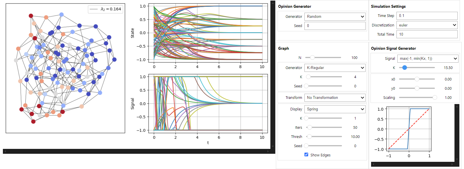
COSA-Simulator is an interactive Jupyter Notebook for studying consensus and polarization in multi-agent systems with nonlinear interactions. It allows researchers and students to visually and intuitively explore the dynamics of networked agents. Users can manipulate network topology, define custom nonlinear signal functions, and observe the system’s evolution in real-time, making it an effective tool for both research and educational purposes.

Interface overview

---

1. Scientific Context

The simulator implements the Continuous Opinion Signaled Action (COSA) dynamics. It is a consensus-like dynamics studied where agents learn not from their neighbors’ opinions, but from their peers’ actions.

On an undirected graph with adjacency matrix \(A\) and degree matrix \(D = \text{diag}(\sum_j A_{ij})\), each agent \(i\) updates its state according to:

\[\Large \dot{x}_i(t) = \frac{1}{d_{i}} \sum_{j \in \mathcal{N}_i} A_{ij} s(x_j(t)) - x_i(t)\]

or in compact matrix form:

\[\Large \dot{x}(t) = D^{-1}A s(x(t)) - x(t)\]

Key elements of this model include:

• \(x(t) = [x_1(t), \dots, x_N(t)]^T \in \mathbb{R}^N\): A vector representing the continuous internal state (opinion) of each agent at time \(t\).
• \(s(\cdot)\): A general, non-decreasing nonlinear signal function that models how agents perceive or communicate their states (signaled action). This can represent phenomena like estimation biases, saturation, or quantization effects.
• \(D^{-1}A\): The normalized adjacency matrix of the network, which defines the topology of agent interactions.

Theoretical Findings: Consensus & Polarization

As established in Couthures et al. (IEEE L-CSS 2025):

1. Synchronization Equilibria: Synchronization equilibria correspond to the fixed points of the signal function \(s(\cdot)\): \[s(x^*) = x^*\] Their stability is determined by the local behavior (underestimation or overestimation) of the signal around these points:
   • If \(s'(x^*) < 1\) (underestimation around \(x^*\)), the synchronized consensus state is locally stable.
   • If \(s'(x^*) > 1\) (overestimation around \(x^*\)), the homogeneous state is unstable / repelling.
2. Emergence of Polarization: Additional research establishes when polarization emerges: when the product of the connectivity measure of the graph \(\lambda_{N-1}(D^{-1}A)\) and the amplification factor \(K\) of the signal function is sufficiently high, i.e.: \[\lambda_{N-1}(D^{-1}A) K > 1\]

This simulator provides a hands-on environment to test and visualize these theoretical findings.

---

2. Interactive Web Demo

Experience the dynamics directly in your browser below. Adjust the network topology, signal function, gain \(K\), and initial states to observe the transition between consensus and polarization in real time. With the stochastic block model, the network has three communities: above the threshold, the agents polarize along them, which is the mechanism behind the SLCD Simulator.

import {makeGraph, sbm, mulberry32, forceLayout, drawNetwork, opinionColor} from "./slcd/slcd.js"

Simulator Controls & Parameters

viewof topology = Inputs.select(
  ["Ring / Circle", "Complete Graph", "Line Graph", "4-Regular Graph", "Erdős–Rényi (p=0.35)", "Stochastic block model (3 × 30)"],
  {value: "Ring / Circle", label: "Topology"}
)

viewof signalType = Inputs.select(
  [
    "Hyperbolic Tangent (tanh)",
    "Saturation / K-Linear",
    "Arctangent (arctan)",
    "Deadzone (δ=0.25)",
    "Two-Plateaux / Multi-cluster"
  ],
  {value: "Hyperbolic Tangent (tanh)", label: "Signal s(x)"}
)

viewof slopeK = Inputs.range([0.2, 3.5], {value: 1.8, step: 0.1, label: "Gain (K)"})

// The block model has a fixed size (3 blocks of 30 agents), as on the SLCD page.
viewof numNodes = Inputs.range([8, 60], {value: 24, step: 2, label: "Agents (N)", disabled: topology === "Stochastic block model (3 × 30)"})

viewof initDist = Inputs.select(
  ["Uniform [-1, 1]", "Bipolar Clusters", "Perturbed Zero"],
  {value: "Uniform [-1, 1]", label: "Initial States"}
)

viewof timeHorizon = Inputs.range([20, 100], {value: 50, step: 5, label: "Horizon (T)"})

viewof reseedBtn = Inputs.button("🎲 New Realization")

function evalSignal(x, type, K) {
  let y = x;
  if (type === "Hyperbolic Tangent (tanh)") {
    y = Math.tanh(K * x);
  } else if (type === "Saturation / K-Linear") {
    y = Math.max(-1.0, Math.min(1.0, K * x));
  } else if (type === "Arctangent (arctan)") {
    y = (2.0 / Math.PI) * Math.atan(K * x);
  } else if (type === "Deadzone (δ=0.25)") {
    const delta = 0.25;
    y = Math.abs(x) > delta ? x : 0.0;
  } else if (type === "Two-Plateaux / Multi-cluster") {
    // Smooth 2-plateaux saturation function strictly bounded in [-1, 1]
    y = 0.5 * Math.tanh(K * (x - 0.5)) + 0.5 * Math.tanh(K * (x + 0.5));
  }
  return Math.max(-1.0, Math.min(1.0, y));
}

// Network topology as an undirected graph (see slcd/slcd.js, shared with the SLCD simulator)
function buildGraph(N, topType, seedVal) {
  if (topType === "Stochastic block model (3 × 30)") {
    // Same parameters as the SLCD simulator: p_in = 0.42, p_out = 0.02.
    const g = sbm(3, 30, 0.42, 0.02, seedVal);
    g.groups = ["Block 1", "Block 2", "Block 3"];
    return g;
  }
  const edges = [];
  if (topType === "Complete Graph") {
    for (let i = 0; i < N; i++) for (let j = i + 1; j < N; j++) edges.push([i, j]);
  } else if (topType === "Line Graph") {
    for (let i = 0; i < N - 1; i++) edges.push([i, i + 1]);
  } else if (topType === "Ring / Circle") {
    for (let i = 0; i < N; i++) edges.push([i, (i + 1) % N]);
  } else if (topType === "4-Regular Graph") {
    for (let i = 0; i < N; i++) edges.push([i, (i + 1) % N], [i, (i + 2) % N]);
  } else {
    // Erdős–Rényi with p = 0.35; an isolated agent is linked to its successor
    const rand = mulberry32(seedVal);
    const deg = new Array(N).fill(0);
    for (let i = 0; i < N; i++) {
      for (let j = i + 1; j < N; j++) {
        if (rand() < 0.35) { edges.push([i, j]); deg[i]++; deg[j]++; }
      }
    }
    for (let i = 0; i < N; i++) if (deg[i] === 0) edges.push([i, (i + 1) % N]);
  }
  return makeGraph(N, edges, new Array(N).fill(0), {groups: ["Agents"]});
}

// Dense row-normalized matrix D^-1 A of a graph
function buildMatrix(g) {
  const W = Array.from({length: g.n}, () => new Float64Array(g.n));
  g.edges.forEach(([u, v], k) => { W[u][v] += g.weight[k]; W[v][u] += g.weight[k]; });
  for (const row of W) {
    const d = row.reduce((a, b) => a + b, 0);
    if (d > 0) for (let j = 0; j < row.length; j++) row[j] /= d;
  }
  return W;
}

// Generate initial opinions - strictly clamped to [-1.0, 1.0]
function getInitialConditions(N, distType, seedVal) {
  let s = Math.abs(Math.sin(seedVal * 12.9898 + 78.233)) * 100000;
  function rand() {
    s = (s * 9301 + 49297) % 233280;
    return (s >>> 0) / 233280; // Strictly in [0, 1)
  }
  const x0 = new Float64Array(N);
  for (let i = 0; i < N; i++) {
    let val = 0;
    if (distType === "Uniform [-1, 1]") {
      val = -0.9 + 1.8 * rand(); // strictly in [-0.9, +0.9]
    } else if (distType === "Bipolar Clusters") {
      const center = (i % 2 === 0) ? 0.65 : -0.65;
      val = center + 0.2 * (rand() - 0.5); // strictly in [-0.75, -0.55] & [0.55, 0.75]
    } else {
      // Perturbed Zero
      val = 0.25 * (rand() * 2 - 1); // strictly in [-0.25, 0.25]
    }
    // Hard clamp to guarantee strictly within [-1.0, 1.0]
    x0[i] = Math.max(-1.0, Math.min(1.0, val));
  }
  return x0;
}

// Network topology and initial condition realization
networkAndInit = {
  reseedBtn; // dependency on button click
  const N = numNodes;
  const top = topology;
  const dist = initDist;
  const seedVal = Math.floor(Math.random() * 1000000);

  const graph = buildGraph(N, top, seedVal);
  const W = buildMatrix(graph);
  const x0 = getInitialConditions(graph.n, dist, seedVal);
  return { N: graph.n, top, dist, graph, W, x0 };
}

// Run simulation
simulationRun = {
  const { N, W, x0 } = networkAndInit;
  const K = slopeK;
  const type = signalType;
  const T = timeHorizon;
  const dt = 0.08;

  let currentX = new Float64Array(x0);

  const traj = [];
  for (let i = 0; i < N; i++) {
    traj.push({ step: 0, time: 0, agent: i, x: currentX[i] });
  }

  // Numerical integration
  const steps = Math.round(T / dt);
  for (let s = 1; s <= steps; s++) {
    const nextX = new Float64Array(N);
    for (let i = 0; i < N; i++) {
      let acc = 0.0;
      for (let j = 0; j < N; j++) {
        if (W[i][j] > 0) {
          acc += W[i][j] * evalSignal(currentX[j], type, K);
        }
      }
      const raw = currentX[i] + dt * (acc - currentX[i]);
      nextX[i] = Math.max(-1.0, Math.min(1.0, raw));
    }
    currentX = nextX;
    if (s % 2 === 0 || s === steps) {
      const curTime = +(s * dt).toFixed(2);
      for (let i = 0; i < N; i++) {
        traj.push({ step: s, time: curTime, agent: i, x: currentX[i] });
      }
    }
  }
  return traj;
}

// Generate data for s(x) curve vs y = x diagonal
signalCurveData = {
  const K = slopeK;
  const type = signalType;
  const pts = [];
  const Npts = 120;
  for (let i = 0; i <= Npts; i++) {
    const x = -1.2 + (2.4 * i) / Npts;
    const sx = evalSignal(x, type, K);
    pts.push({ x: +x.toFixed(3), sx: +sx.toFixed(3), diag: +x.toFixed(3) });
  }
  return pts;
}

Signal Function & Fixed Points

Synchronization equilibria at \(x = s(x)\).

Plot.plot({
  width: 360,
  height: 360,
  aspectRatio: 1,
  x: { label: "Agent State x", domain: [-1.2, 1.2], grid: true },
  y: { label: "Communicated Signal s(x)", domain: [-1.2, 1.2], grid: true },
  marks: [
    Plot.ruleX([0], { stroke: "#cccccc" }),
    Plot.ruleY([0], { stroke: "#cccccc" }),
    // Diagonal y = x
    Plot.line(signalCurveData, {
      x: "x",
      y: "diag",
      stroke: "#94a3b8",
      strokeDasharray: "4,4",
      strokeWidth: 1.5
    }),
    // Signal curve s(x)
    Plot.line(signalCurveData, {
      x: "x",
      y: "sx",
      stroke: "#0d6efd",
      strokeWidth: 2.5
    })
  ]
})

— Blue curve: Nonlinear signal \(s(x)\)
- - Dashed line: Reference diagonal \(y=x\)

Time Evolution \(x_i(t)\) of Networked Agents

Agent state trajectories showing convergence or clustering.

Plot.plot({
  height: 430,
  x: { label: "Time t", grid: true },
  y: { label: "State x_i(t)", domain: [-1.2, 1.2], grid: true },
  // Each curve takes the colour of its agent's final state, as on the network below.
  color: { type: "identity" },
  marks: [
    Plot.ruleY([0], { stroke: "#e2e8f0" }),
    Plot.line(simulationRun, {
      x: "time",
      y: "x",
      z: "agent",
      stroke: (d) => opinionColor(cosaFrames[cosaFrames.length - 1].x[d.agent]),
      strokeWidth: 1.8,
      strokeOpacity: 0.8
    })
  ]
})

— Colored curves: Agent state trajectories \(x_i(t)\), coloured by final state (blue −1, grey 0, red +1)
• Asymptotic state: Convergence to consensus or cluster partitions

The Network

The graph of the current realization. Node colour shows the final state of each agent; press ▶ to replay the dynamics.

cosaLayout = forceLayout(d3, networkAndInit.graph)

// States x(t) of every agent at each recorded time.
cosaFrames = d3.groups(simulationRun, (d) => d.time).map(([time, rows]) => {
  const x = new Float64Array(networkAndInit.N);
  for (const r of rows) x[r.agent] = r.x;
  return {time, x};
})

cosaNetwork = {
  const g = networkAndInit.graph, frames = cosaFrames;
  const isSbm = g.groups.length > 1;
  const W = Math.max(320, Math.min(width, 980)), H = Math.round(W * (W < 600 ? 0.9 : 0.5));
  // Same node size for every topology.
  const {svg, lines, circles} = drawNetwork(d3, g, cosaLayout, {width: W, height: H, padRight: W >= 576 ? 170 : 14, radius: 7});
  lines.attr("stroke", "var(--slcd-edge)").attr("stroke-width", 1).attr("stroke-opacity", 0.7);
  circles.attr("stroke", "none");
  const titles = circles.append("title");

  const legend = html`<div class="slcd-legend"></div>`;
  const show = (f) => {
    const {time, x} = frames[f];
    circles.attr("fill", (i) => opinionColor(x[i]));
    titles.text((i) => `Agent ${i + 1}${isSbm ? ` (${g.groups[g.labels[i]]})` : ""}\nx = ${x[i].toFixed(3)}`);
    legend.innerHTML = `<div class="slcd-legend-title">t = ${time.toFixed(1)}</div>`
      + `<div class="slcd-legend-row"><span class="slcd-ramp"></span>State −1 … +1</div>`;
  };

  const button = cosaReplay.querySelector("button");
  let timer = null;
  const stop = () => { clearInterval(timer); timer = null; button.textContent = "▶ Replay the dynamics"; show(frames.length - 1); };
  // Log-spaced frames: the transient is fast, the convergence slow.
  const last = frames.length - 1;
  const order = [0, ...new Set(d3.range(1, 151).map((j) => Math.round(Math.exp((Math.log(last) * j) / 150))))];
  button.onclick = () => {
    if (timer) return stop();
    let f = 0;
    button.textContent = "■ Stop";
    timer = setInterval(() => {
      show(order[f]);
      if (++f >= order.length) stop();
    }, 50);
  };
  invalidation.then(() => { clearInterval(timer); button.textContent = "▶ Replay the dynamics"; });

  show(frames.length - 1);
  return html`<div class="slcd-network-box">${svg.node()}${legend}</div>`;
}

cosaReplay = html`<div class="slcd-replay">
  <button type="button" class="slcd-play">▶ Replay the dynamics</button>
  <span>Time runs on a logarithmic scale, so the fast start of the dynamics stays visible.</span>
</div>`

---

3. Features

• Interactive Simulation: A user-friendly interface built with ipywidgets allows for real-time control over all simulation parameters without rewriting code.
• Network Generation:
  • Generate standard network topologies like K-Regular, Complete, and Line graphs.
  • Use a random seed for reproducible experiments.
• Nonlinear Signal Control:
  • Define a wide range of monotonic, Lipschitz-continuous signal functions \(s(\cdot)\).
  • Interactively adjust parameters (e.g., gain K, offsets) and immediately visualize the function’s shape.
  • Includes presets for common functions like linear, affine, and sigmoidal/saturation models.
• Rich Visualization:
  • View the network graph with nodes colored according to their state.
  • Plot the time evolution of each agent’s state and signal.
  • Analyze convergence towards synchronization equilibria.
• Data Export:
  • Save simulation trajectories and results to CSV files.
  • Export plots as high-quality PNG images for use in manuscripts and presentations.

---

4. Getting Started

Prerequisites

• Python 3.9 or higher
• JupyterLab or Jupyter Notebook

Installation & Launch

Follow these steps to set up and run the simulator:

1. Clone the repository:

   git clone https://github.com/AnthonyCouthures/COSA-Simulator.git
   cd COSA-Simulator

2. Create and activate a virtual environment:

   # Create the environment
   conda create -n "COSA_Simulator" python=3.11.15 ipython
   
   # Activate it 
   conda activate COSA_Simulator

3. Install the required dependencies:

   pip install -r requirements.txt

4. Open and run the notebook: Navigate to COSA - Simulator/ and open Interface.ipynb. Execute the cells in order to launch the interactive interface.

---

5. Repository Structure

The repository is organized to separate the user interface from the core simulation logic:

COSA-Simulator/
│   ├── interface.ipynb     # The main Jupyter notebook with the interactive UI.
│   ├── __init__.py         # Makes the Simulator directory a Python package.
│   └── ...                 # Core Python modules for simulation, graphing, etc.
├── requirements.txt        # A list of Python package dependencies.
├── LICENSE
└── README.md

For the simulator to function correctly, the Simulator package must be importable by the Interface.ipynb notebook. Always run Jupyter from the root of the repository.

---

6. Reproducibility & Contributing

To ensure your experiments are reproducible: * Set the Seed: Always use a specific integer seed in the UI for any experiment that relies on random generation (e.g., initial conditions, graph topology). * Pin Versions: The requirements.txt file should contain pinned versions of libraries to avoid issues from upstream updates.

---

7. How to Cite

If you use this simulator in your research, please cite the accompanying paper and the software itself:

Paper:

@article{couthures2025global,
  title = {Global Synchronization of Multi-Agent Systems With Nonlinear Interactions},
  author = {Couthures, Anthony and Varma, Vineeth S. and Lasaulce, Samson and Morărescu, Irinel-Constantin},
  year = {2025},
  journal = {IEEE Control Systems Letters},
  volume = {9},
  pages = {354--359},
  issn = {2475-1456},
  doi = {10.1109/LCSYS.2025.3573563},
  url = {https://ieeexplore.ieee.org/document/11015590}
}

Software:

@software{anthony_couthures_2025_17407391,
  author       = {Anthony Couthures},
  title        = {AnthonyCouthures/COSA-Simulator: First Release},
  month        = oct,
  year         = 2025,
  publisher    = {Zenodo},
  version      = {Main},
  doi          = {10.5281/zenodo.17407391},
  url          = {https://doi.org/10.5281/zenodo.17407391}
}

---

8. License

This project is licensed under the MIT License. See the LICENSE file on GitHub for details.